This article was created by pure chance. A few days ago, while organizing the bookcase, I found my notes from the Hydraulic Infrastructures course I took when I was an engineering student. Along with those notes there was also the report, calculations, graphs and drawings of the aqueduct project to be discussed in the exam. The very first steps were precisely the search for the best point in which to position the tank serving the internal network and the identification of the route for the approach pipeline. Below I will explain how it is possible with QGIS to define these two design variables that sit at the basis of aqueduct design.
NB: the aim of this article is not to be a step-by-step tutorial; it is purely informative.
At the university I remember that we were given a IGM 1:25,000 map on which the municipality to be served and the source from which to draw the water were identified. With only this data we identified (I speak in the plural because I was in a working group) the height of the tank and with the help of the isoipses we defined the route with the relative altimetric profile. In reality the most It was annoying and time-consuming to identify the route and define the altitude profile because we went to identify 3-4 solutions. In the end we chose the one that seemed least burdensome from the point of view of both excavation and expropriation costs as well as the length of the route itself. I remember that to calculate the altitude profile we used a command line application, it looked like DOS, in which we inserted the data we had detected on the IGM card and at the end he drew it for us. the altimetric profile by entering the progressive and absolute distance section by section as well as the slope.
Once the romantic excursus is over, let's get to the point!

The situation at the start of the project is this:
- source at an altitude of 444 metres;
- tank height, calculated taking into account the maximum height of the town to be served, the height of the highest building high, load losses of 430 metres.
In addition to these data and the IGM map I used the DTM of the ISPRA with a resolution of 20 meters per pixel. I reclassified a clip of the study area according to three altimetric bands:
- Class 0: altitudes between the minimum altitude of the clip and altitude 427 metres;
- Class 1: altitudes between 428 and 432 metres;
- Class 2: altitudes between 433 meters and the maximum altitude of the clip.
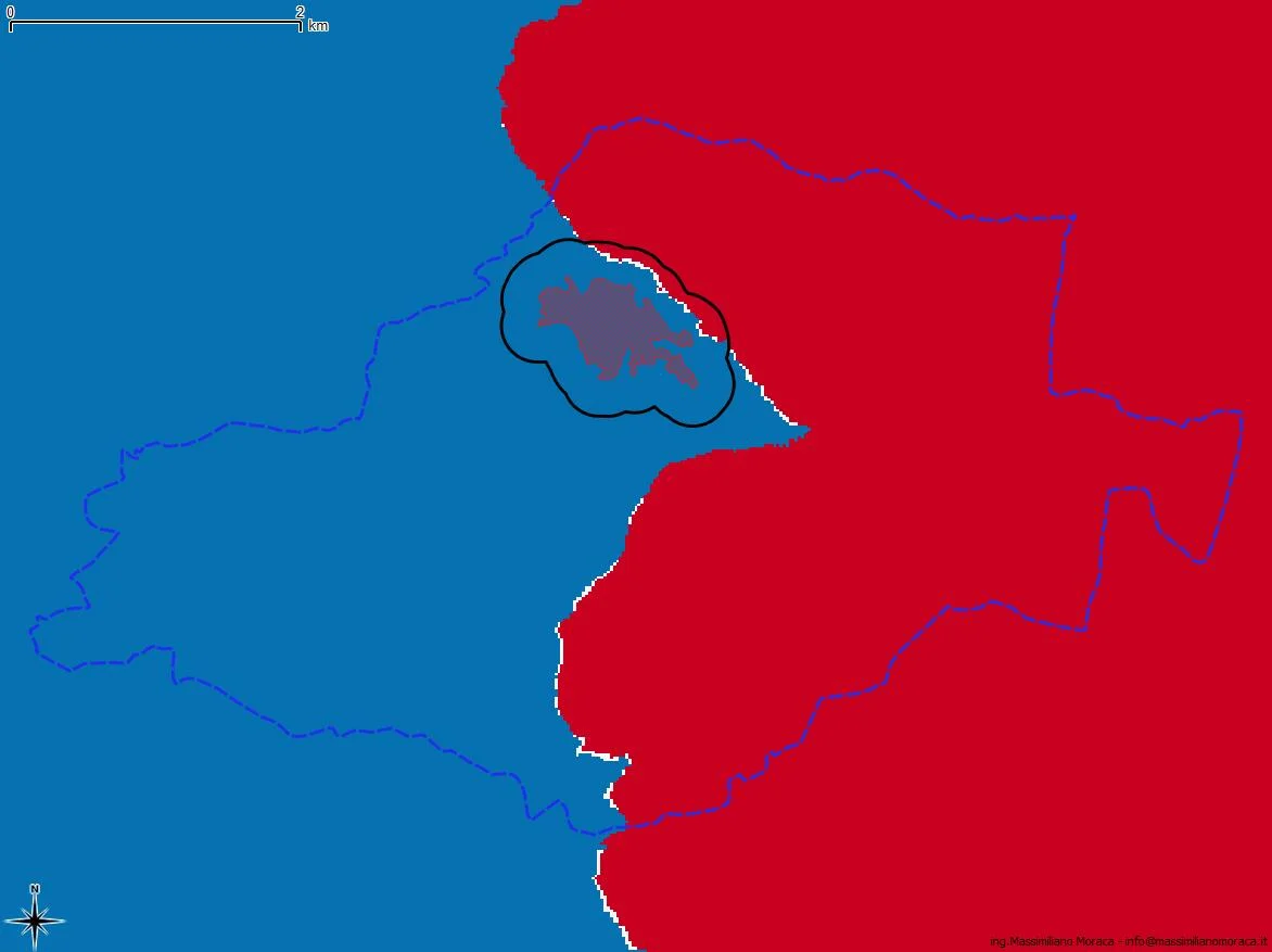 The class I'm interested in is the 1 which includes the height of the tank +/- 2 metres. By overlaying the reclassified raster with a buffer 250 meters from the town center it will be possible to possible to identify the best area to place the tank. The white pixels are those in correspondence with areas useful for this purpose.
Having identified the best area to position the tank, I moved on to the next step: tracing the route of the approach pipeline.
In the video I explain all the steps I took until I identified the route itself.
Once I knew the path, I used the qProf plugin to trace the altitude profile with progressive distance between positive and negative cusps, total distance and slope of the sections. It is important to know that the profile obtained is depending on the resolution of the DEM from which it originates. If you have a DEM at 1m/px the result will be certainly better than mine at 20m/px.
In the following video I explain how to obtain the altitude profile and export it as csv to then be processed in a spreadsheet.
The exercise is finished, see you next time :)
NB: the data to repeat the exercise is attached.